


A GAN, or Generative Adversarial Network, is a machine learning model that creates new data by training two neural networks against each other. One network generates new samples. The other network judges how real those samples look. The two networks compete, and this competition pushes both to improve.
Ian Goodfellow and his colleagues introduced GANs in 2014, and the idea changed how computers create content. Earlier generative models produced blurry or vague output. GANs learned to produce sharp images of faces, animals, buildings, and artwork. Websites such as This Person Does Not Exist display faces of people who do not exist, and every face comes from a GAN.
The rest of this page covers what a GAN is, how it works, and where it breaks down. It includes the exact hyperparameters researchers use, a full training-loop walkthrough, and an honest comparison with diffusion models — including the trade-offs that generic explainers usually leave out.
What Is a Generative Adversarial Network?
A Generative Adversarial Network is a deep learning framework where a generator network and a discriminator network train together in a two-player game. The generator creates synthetic data, such as images or audio. The discriminator evaluates that data and decides whether each sample is real or fake.
The framework belongs to a field called generative modeling. Generative models learn the patterns inside a dataset and then produce new samples that follow those same patterns. A generative model trained on 50,000 photographs of cats learns what cats look like and can then draw a new cat that appeared in none of the training photos.
Two words in the name describe the system. “Generative” means the model generates new data. “Adversarial” means the two networks act as opponents. Each network has a goal that works against the other network. This opposition is the core design, and it drives the learning process.
A GAN needs three parts to function:
- A generator that produces candidate samples from random inputs
- A discriminator that scores each sample as real or fake
- A training set of real data, such as photographs, drawings, or audio clips
The networks train at the same time. Neither network works alone. The generator improves because the discriminator finds its flaws. The discriminator improves because the generator produces harder fakes.
How Does a GAN Work?
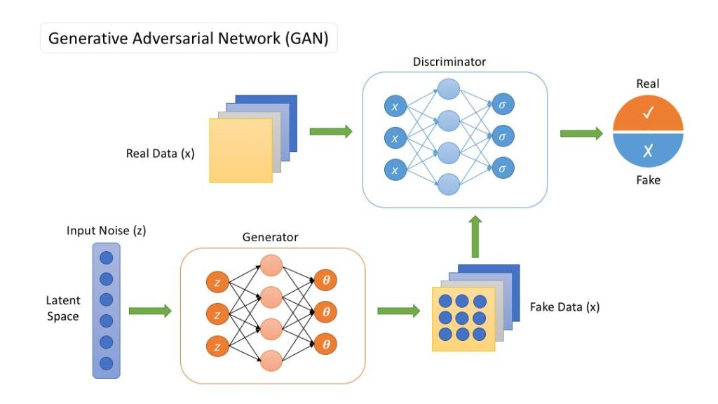
A GAN works by running a repeated loop where the generator creates fake samples, the discriminator judges them, and both networks update their internal settings based on the results. Each round of this loop makes the generator harder to catch and the discriminator harder to fool.
The process follows five steps:
- The generator receives a random number vector, called a latent vector, and converts it into a sample, such as a 64 by 64 pixel image.
- The training set supplies real samples. A common example is the MNIST dataset, which contains 70,000 images of handwritten digits.
- The discriminator receives a mix of real and generated samples.
- The discriminator outputs a probability score for each sample. A score near 1 means “real,” and a score near 0 means “fake.”
- Both networks update their weights. The generator learns from the discriminator’s feedback and adjusts its output. The discriminator learns from its own mistakes.
This loop repeats thousands or millions of times. Early in training, the generator produces noise that looks like static. As training continues, the noise gains structure. First comes a rough shape, then edges, then colors, and finally clear details. A well-trained GAN produces images that human reviewers struggle to separate from real photographs.
What Does the Generator Do?
The generator creates new synthetic samples from random noise, and its goal is to produce output that the discriminator labels as real. The generator never sees the real training data directly. It learns about the data only through the discriminator’s judgment.
The generator starts with a latent vector. This vector is a list of random numbers, often 100 values, drawn from a simple distribution. The network transforms this list through many layers of mathematical operations. Each layer adds structure. In an image generator, early layers set the rough layout, middle layers add shapes, and final layers add texture and fine detail.
The generator’s success depends entirely on the discriminator. If the discriminator rejects its output, the generator adjusts its internal parameters and tries again. Over many rounds, the generator maps regions of random noise to specific features. One region may control hair color, another may control the angle of a face, and another may control background lighting.
What Does the Discriminator Do?
The discriminator classifies samples as real or fake, and its goal is to label every generated sample as fake and every training sample as real. The discriminator is a standard classifier, similar to networks used for spam detection or object recognition.
The discriminator receives samples from two sources. The first source is the training set, and the second source is the generator. It outputs a single probability score for each sample. During training, two forces act on the discriminator. It must reject fakes from the generator, and it must accept genuine samples from the dataset.
The discriminator acts as a teacher for the generator. Because it produces a score rather than a simple verdict, its feedback contains direction. The generator can calculate which small change would raise its score. This gradient feedback is what allows the generator to learn without ever seeing real data directly.
Why Did Researchers Develop GANs?
Ian Goodfellow and his colleagues developed GANs in 2014 to solve a core problem in generative modeling. Their paper, “Generative Adversarial Networks,” appeared at the NeurIPS conference, and the work has earned more than 100,000 citations.
Earlier generative approaches had two main branches, and each branch had limits. The first branch used explicit density models, such as variational autoencoders. These models computed the probability of the data, but they often produced blurry samples. The second branch avoided explicit probability calculations, but many of those methods were unstable or inflexible.
GANs took a different path. They avoided explicit probability calculations and learned through competition instead. The result was a model that could generate sharp, realistic samples. The original paper used simple datasets such as MNIST and the Toronto Face Dataset. The idea scaled far beyond those early tests in the following decade.
What Is the GAN Minimax Objective?
The GAN minimax objective is a mathematical function that both networks try to optimize in opposite directions. The generator tries to minimize it, and the discriminator tries to maximize it. This push in opposite directions creates the adversarial game.
The formula is written as min over G of max over D of V(D, G). The value V combines two parts. The first part is the log probability that the discriminator assigns to real data. The second part is the log probability of the opposite verdict for generated data.
In plain words, the discriminator wins points for correct answers. The generator wins points for wrong answers given by the discriminator. Goodfellow’s paper showed that this game reaches a theoretical optimum when the generated data distribution exactly matches the real data distribution. At that point, the discriminator is correct 50 percent of the time, which is the same as random guessing.
Reaching that perfect balance is difficult. The two networks improve at different speeds. This imbalance causes most of the training problems covered later on this page.
What Are the Main Types of GAN Architectures?
The main GAN architectures include DCGAN, WGAN, CycleGAN, and StyleGAN, and each one extends the original 2014 design to solve a specific weakness or task. Researchers have published hundreds of GAN variants. The four below are the most influential, with two additional types worth knowing.
1. DCGAN (Deep Convolutional GAN)
DCGAN applies convolutional neural networks to both the generator and the discriminator. Alec Radford, Luke Metz, and Soumith Chintala introduced it in 2015, and their paper has gathered more than 22,000 citations. DCGAN established design rules that made GAN training far more stable:
- Replace pooling layers with strided convolutions, so the network learns its own downsampling
- Use batch normalization in most layers of both networks
- Remove fully connected hidden layers on top of convolutional features
- Use ReLU activations in the generator and LeakyReLU activations in the discriminator
The paper’s training recipe is specific: a mini-batch size of 128, the Adam optimizer with a learning rate of 0.0002, and the Adam momentum term beta1 set to 0.5 instead of the default 0.9. That single change to beta1 matters — the authors found the standard 0.9 caused training to oscillate and stall. This recipe is still the default starting point in the official PyTorch DCGAN tutorial.
2. WGAN (Wasserstein GAN)
WGAN replaces the original loss function with the Wasserstein distance, also called the earth mover’s distance. Martin Arjovsky and colleagues introduced it in 2017, and the paper states that this change improves training stability and reduces mode collapse. The practical recipe calls for clipping the critic’s weights to the range [-0.01, 0.01] and updating the critic 5 times for every 1 generator update. The term “critic” replaces “discriminator” in this paper, because the network now outputs an unbounded score instead of a probability. WGAN also produces loss values that track image quality, which gives developers a useful training signal — a luxury the original loss never offered.
3. CycleGAN
CycleGAN translates images from one domain into another without paired training examples. Jun-Yan Zhu and colleagues introduced it in 2017. The model learns to convert horses into zebras, summer scenes into winter scenes, and paintings into photographs. Its key innovation is the cycle consistency loss. If the model converts a horse into a zebra, converting the result back should return the original horse. CycleGAN has earned more than 34,000 citations.
4. StyleGAN
StyleGAN changes the generator architecture to give researchers fine control over generated images. Tero Karras and the NVIDIA team introduced it in 2018. The style-based generator injects style information at every layer, which allows separate control of coarse features, such as face shape, and fine features, such as skin texture. StyleGAN and its successors, including StyleGAN2 and StyleGAN3, produce some of the most realistic synthetic faces available. The website This Person Does Not Exist runs on this family of models.
Other Notable Variants
Two more types appear often in research and production:
- Conditional GAN (cGAN): Generates samples that match a given label, such as “generate a digit 7”
- Progressive GAN: Grows the image resolution in steps during training, which enables high-resolution output
How Do GANs Compare With VAEs and Diffusion Models?
GANs, VAEs, and diffusion models are the three main families of deep generative models for images. GANs produce the fastest samples, VAEs offer the most stable training, and diffusion models currently produce the highest quality and diversity.
| Feature | GAN | VAE | Diffusion Model |
|---|---|---|---|
| Sample speed | Fast, usually 1 network pass | Fast, 1 network pass | Slow, hundreds of denoising steps |
| Image quality | High, sharp output | Moderate, often blurry | Very high |
| Training stability | Low, two networks compete | High, single objective | High, single objective |
| Output diversity | Limited by mode collapse risk | High | Very high |
| Likelihood score | Not available | Available | Available |
| Best known examples | StyleGAN2, DCGAN, CycleGAN | VAE, β-VAE | Stable Diffusion, DALL-E |
The speed gap deserves a concrete number. A GAN produces one image in a single forward pass through the generator. A diffusion model runs the same kind of network 20 to 1,000 times, refining the image a little on each pass. For a design tool that redraws an image while the user drags a slider, only the GAN responds fast enough.
Each family fits different needs. Use GANs when speed matters, such as real-time image editing. Use VAEs when a stable model or a compact data representation matters more than sharpness. Use diffusion models when maximum quality and diversity matter and generation speed does not. Diffusion models have taken over many text-to-image products since 2022, but GANs remain common in research, editing tools, and applications that need instant output.
What Are GANs Used For?
GANs generate, edit, and enhance data across many industries. The most common applications include the following:
- Generate synthetic images for design, art, and advertising
- Create artificial training data for other machine learning models
- Perform image-to-image translation, such as converting sketches into photos
- Increase dataset size for medical imaging, where real patient scans are limited
- Produce super-resolution output, which raises the detail level of low-resolution images
- Build realistic video game textures and 3D assets
- Detect deepfakes, since GAN research also improves detection tools
Medical imaging shows why synthetic data matters. Hospitals protect patient privacy, so sharing large scan datasets is difficult. GANs can generate realistic synthetic scans that let researchers develop and test diagnostic models without exposing patient records. Researchers at NVIDIA and the Mayo Clinic published work in 2019 showing that GAN-generated brain MRI images could improve tumor classification models.
Data augmentation works the same way. A self-driving car project may collect thousands of images of pedestrians. GANs can vary lighting, weather, and clothing in those images. The result is a larger and more varied training set at a lower cost.
Why Are GANs Hard to Train?
GANs are hard to train because two networks learn at the same time, and their goals conflict. This conflict produces three well-documented problems: mode collapse, vanishing gradients, and non-convergence.
Mode Collapse
Mode collapse happens when the generator produces a small variety of outputs while ignoring most of the data distribution. A GAN trained on 10 digit classes may only generate 7s and 1s, because the generator found a few outputs that reliably fool the discriminator and keeps reusing them. Google’s machine learning documentation lists mode collapse as a standard GAN failure mode, and the Wasserstein GAN paper was written specifically to reduce it. Practical fixes include the WGAN loss, minibatch discrimination, and lowering the generator’s learning rate so it cannot lock onto one winning output.
Vanishing Gradients
Vanishing gradients happen when the discriminator becomes too strong. A near-perfect discriminator gives the generator almost no useful feedback, so learning slows or stops. If the generator’s fakes are all rejected with high confidence, the signal flowing back to the generator grows too small to guide improvement. The usual fix is to weaken the discriminator on purpose — fewer discriminator updates per round, noisier inputs, or softer labels.
Non-Convergence and Instability
Non-convergence happens when the two networks fall into a cycle. The generator improves, then the discriminator adapts, then the generator must start over. Training loss curves bounce instead of settling. This behavior makes it hard to decide when to stop training and which model checkpoint to keep.
How Do Researchers Address These Problems?
Tim Salimans and colleagues at OpenAI published a set of fixes in 2016 that practitioners still use. The paper’s one-sided label smoothing changes the target for real samples from 1.0 to 0.9, which stops an overconfident discriminator from producing extreme gradients. The same paper introduced feature matching, which trains the generator to match statistics inside the discriminator rather than just flipping its verdict. Beyond that paper, common techniques include the following:
- Apply spectral normalization to stabilize the discriminator
- Use the Wasserstein loss with a gradient penalty coefficient of 10, as in WGAN-GP, which replaced weight clipping in most modern implementations
- Use one-sided label smoothing with a real-label target of 0.9
- Train with a balanced ratio of generator and discriminator updates, such as 5 discriminator updates per generator update in WGAN
- Use batch normalization inside both networks
- Start training at low resolution and increase it in steps, as Progressive GAN does
How Can You Start Building a GAN?
You can build your first GAN with Python, a deep learning library, and a standard dataset. Here is the training loop in pseudocode, which is the part beginners most often get wrong:
for each batch:
    # 1. Train the discriminator on real data
    real_batch = sample from training set
    real_loss = BCE(discriminator(real_batch), label = 1)

    # 2. Train the discriminator on fake data
    noise = random vector, size 100
    fake_batch = generator(noise)
    fake_loss = BCE(discriminator(fake_batch), label = 0)

    # 3. Update discriminator weights only
    update discriminator using (real_loss + fake_loss)

    # 4. Train the generator using the discriminator's feedback
    noise = random vector, size 100
    gen_loss = BCE(discriminator(generator(noise)), label = 1)

    # 5. Update generator weights only
    update generator using gen_loss
Three details in that loop decide whether training works. First, the label in step 4 is 1, not 0 — the generator wants the discriminator to believe its fakes are real. Second, in step 3 the generator must be treated as frozen, and in step 5 the discriminator must be treated as frozen; updating both at once makes the feedback signal meaningless. Third, do not detach gradients carelessly — a common bug is letting the generator’s update flow through stale discriminator weights.
Follow these steps to run a complete project:
- Install a deep learning framework such as PyTorch or TensorFlow. PyTorch and TensorFlow are the two most widely used options.
- Choose a small dataset, such as MNIST, which contains 70,000 grayscale digit images.
- Build a generator network with 3 to 5 layers that maps a 100-value random vector to a 28 by 28 image.
- Build a discriminator network with 3 to 5 layers that maps an image to one probability score.
- Train with binary cross-entropy loss, alternating between generator updates and discriminator updates.
- Inspect generated samples every few hundred steps to watch quality improve.
- Set the Adam optimizer to a learning rate of 0.0002 with beta1 = 0.5, following the DCGAN recipe, if training oscillates or stalls.
A basic MNIST GAN runs on a free cloud GPU or a consumer laptop with a modern graphics card. Training typically takes between 30 minutes and 2 hours. The official PyTorch and TensorFlow documentation both ship complete, working DCGAN code.
Frequently Asked Questions
Is a GAN a type of neural network?
Yes. A GAN is a framework built from two neural networks, the generator and the discriminator. Each network is a standard deep neural network, usually made of convolutional or dense layers. The GAN is not one single network but a system of two networks trained together.
Can a GAN create images of people who do not exist?
Yes. StyleGAN models generate realistic faces of people who have never existed. The website This Person Does Not Exist shows a new synthetic face each time a visitor loads the page. Each face is a statistical blend of patterns learned from training data, not a copy of any real person.
Are GANs still used after diffusion models became popular?
Yes. GANs remain in use where fast generation matters. Diffusion models need hundreds of network passes to produce one image, while a GAN needs one pass. This speed advantage keeps GANs relevant for real-time editing, video games, and interactive design tools. GANs also remain an active research area.
Is training a GAN harder than training other neural networks?
Yes. GAN training involves two competing networks, while a standard classifier trains one network against a fixed dataset. The competition creates instability, mode collapse, and sensitivity to hyperparameters. A beginner can train a basic GAN, but reaching high-quality, diverse output requires more tuning than most supervised models.
Can a GAN work with data other than images?
Yes. GANs generate audio, text, music, and tabular data. Image generation is the most common use because convolutional networks handle images well. Audio examples include voice synthesis and music generation. Text generation GANs exist but perform worse than modern language models because text is discrete and harder to optimize.
Did Ian Goodfellow invent GANs alone?
No. The 2014 GAN paper lists several authors: Ian Goodfellow, Jean Pouget-Abadie, Mehdi Mirza, Bing Xu, David Warde-Farley, Sherjil Ozair, Aaron Courville, and Yoshua Bengio. Goodfellow proposed the core idea and is credited as the lead author, but the work came from a team at the Université de Montréal and related institutions.
Conclusion
A Generative Adversarial Network is a two-network system in which a generator creates synthetic data and a discriminator judges it, and the competition between them produces realistic output. The design turned a simple question — can two networks train each other? — into one of the most influential ideas in modern machine learning.
The key points in one place:
- A GAN contains 2 networks: a generator that creates samples and a discriminator that scores them
- Ian Goodfellow and 7 coauthors introduced the framework in 2014 at NeurIPS
- Key variants include DCGAN (2015), WGAN (2017), CycleGAN (2017), and StyleGAN (2018)
- The 3 main training problems are mode collapse, vanishing gradients, and non-convergence
- Proven fixes exist and come with exact settings: label smoothing to 0.9, a 0.0002 learning rate with beta1 = 0.5, and a gradient penalty of 10 in WGAN-GP
- Compared with VAEs and diffusion models, GANs offer the fastest generation speed but the least stable training
- Common uses include synthetic data, image translation, super-resolution, and medical imaging
GANs no longer dominate text-to-image generation, since diffusion models now lead that field. The adversarial training idea remains fundamental regardless. It teaches how two models can improve each other through competition, and that principle continues to shape new research in generative AI. Anyone who wants to understand how modern AI creates content benefits from learning how GANs work first.
Sources: Goodfellow et al., Generative Adversarial Nets, NeurIPS 2014 · Radford et al., DCGAN, 2015 · PyTorch DCGAN Tutorial · Arjovsky et al., Wasserstein GAN, 2017 · Gulrajani et al., WGAN-GP, NeurIPS 2017 · Salimans et al., Improved Techniques for Training GANs, 2016 · Zhu et al., CycleGAN, 2017 · Karras et al., StyleGAN, 2018 · Google ML GAN failure modes · This Person Does Not Exist
You May Also Like
 SaaS
What Is No-Code Automation? How It Works, Benefits, and Risks
 Web Scraping
TinyFish.ai Review: Is It the Best AI Agent for Web Scraping
 AI Technology
ChatGPT API Alternatives: 13 AI APIs and Platforms for Developers
 Web Development
Building Apps with Lovable and Supabase: A Step-by-Step Guide
 AI Tools
10 Best PDF Extraction APIs for Text, Tables, OCR, and Structured Data
 Web Scraping
What Is AI Web Scraping? A Complete Guide to AI-Powered Data Extraction
 Web Scraping
Scrapy in Python: A Practical Guide to Web Scraping
 AI Tools
15 Best Free AI APIs for Developers: Free Tiers, Credits, and Limits Explained
 AI Technology
